Find Particular Solution to Differential Equation With Step Function
We introduce the unit step function and some of its applications.
The Unit Step Function
In the next section we'll consider initial value problems where , , and are constants and is piecewise continuous. In this section we'll develop procedures for using the table of Laplace transforms to find Laplace transforms of piecewise continuous functions, and to find the piecewise continuous inverses of Laplace transforms.
Use the table of Laplace transforms to find the Laplace transform of
Since the formula for changes at , we write To relate the first term to a Laplace transform, we add and subtract in (eq:8.4.2) to obtain To relate the last integral to a Laplace transform, we make the change of variable and rewrite the integral as
Since the symbol used for the variable of integration has no effect on the value of a definite integral, we can now replace by the more standard and write This and (eq:8.4.3) imply that Now we can use the table of Laplace transforms to find that
Laplace Transforms of Piecewise Continuous Functions
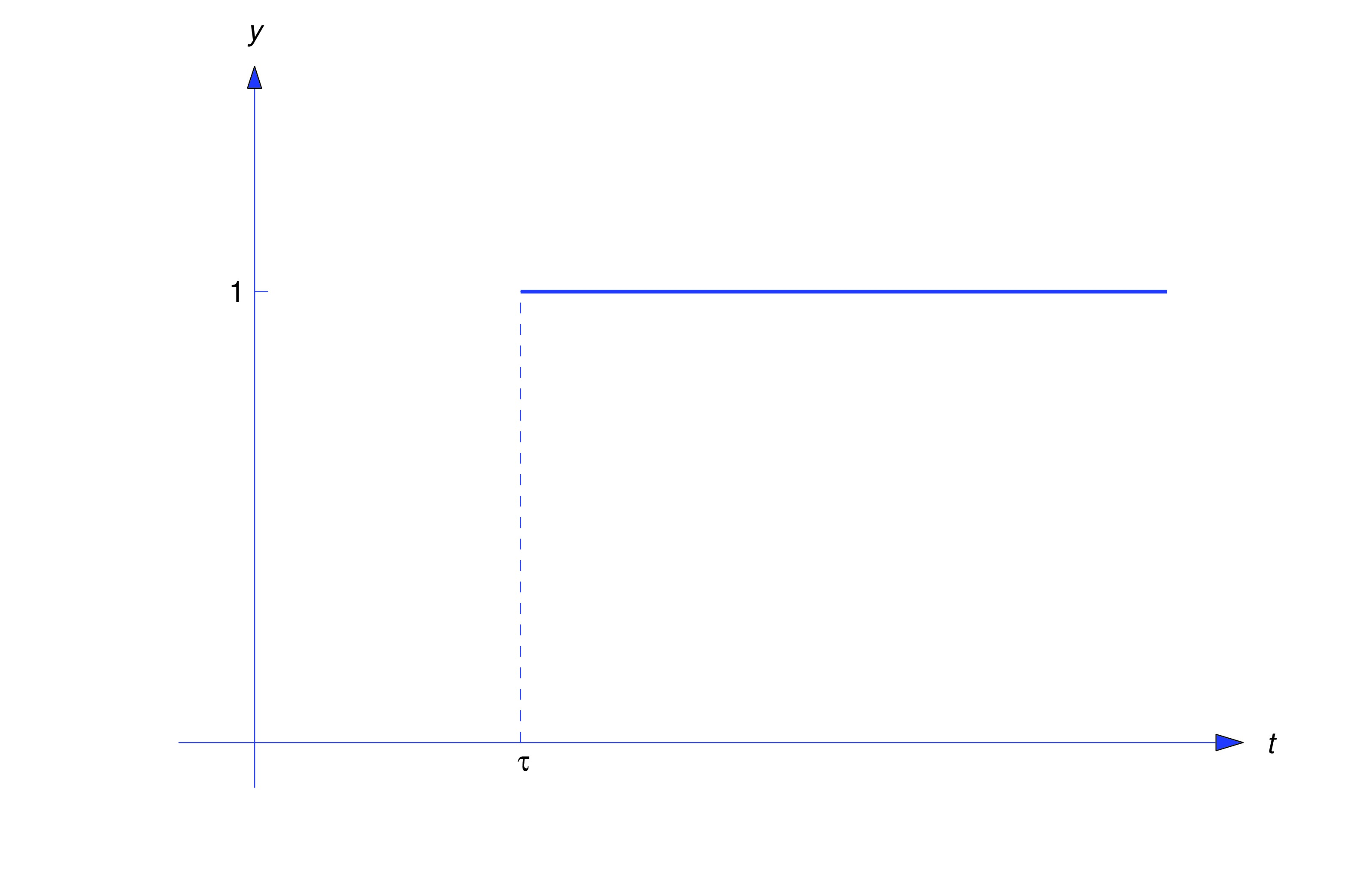
We'll now develop the method of Example example:8.4.1 into a systematic way to find the Laplace transform of a piecewise continuous function. It is convenient to introduce the unit step function, defined as
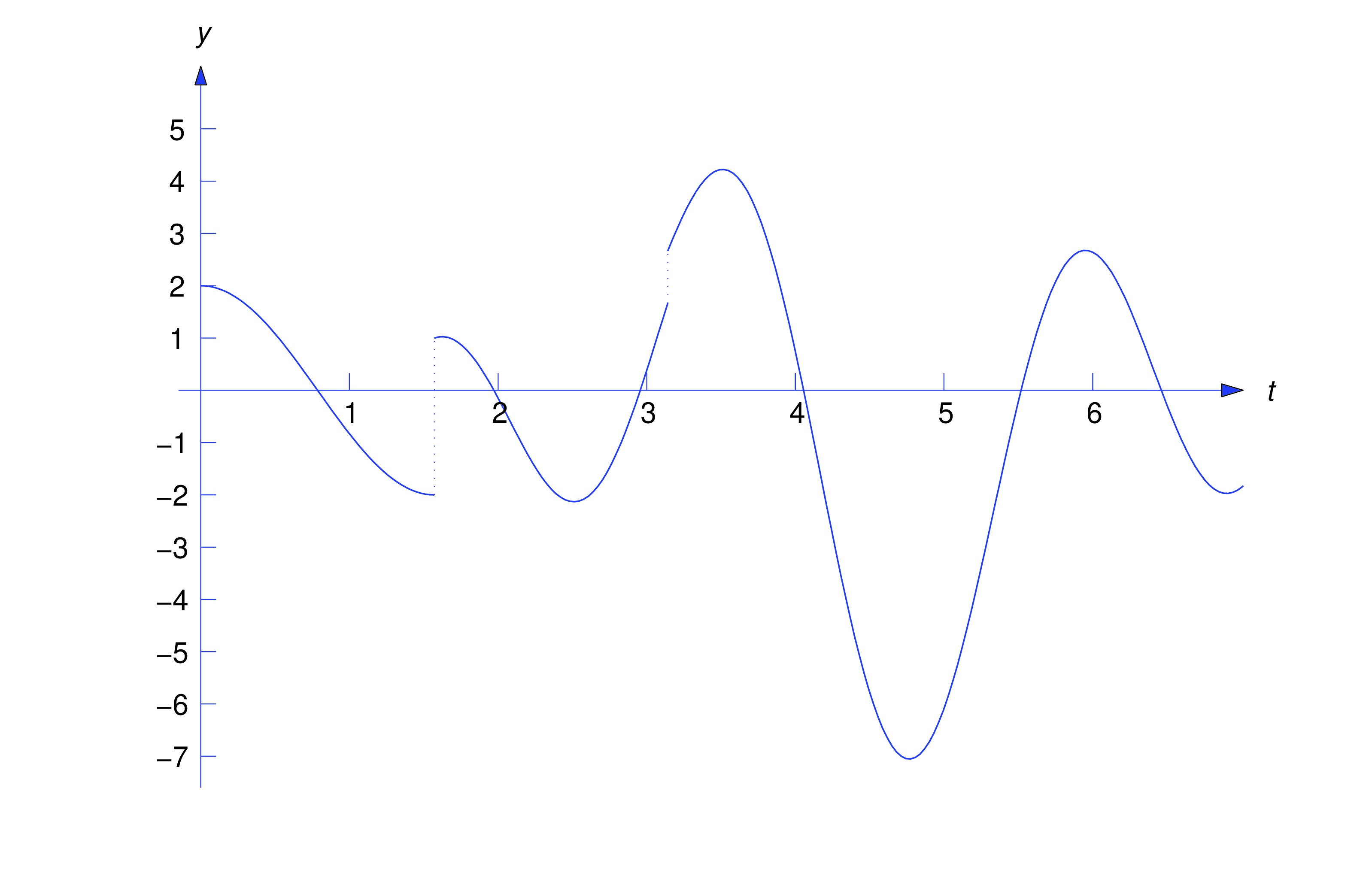
Thus, "steps" from the constant value to the constant value at . If we replace by in (eq:8.4.4), then that is, the step now occurs at (See figure below)
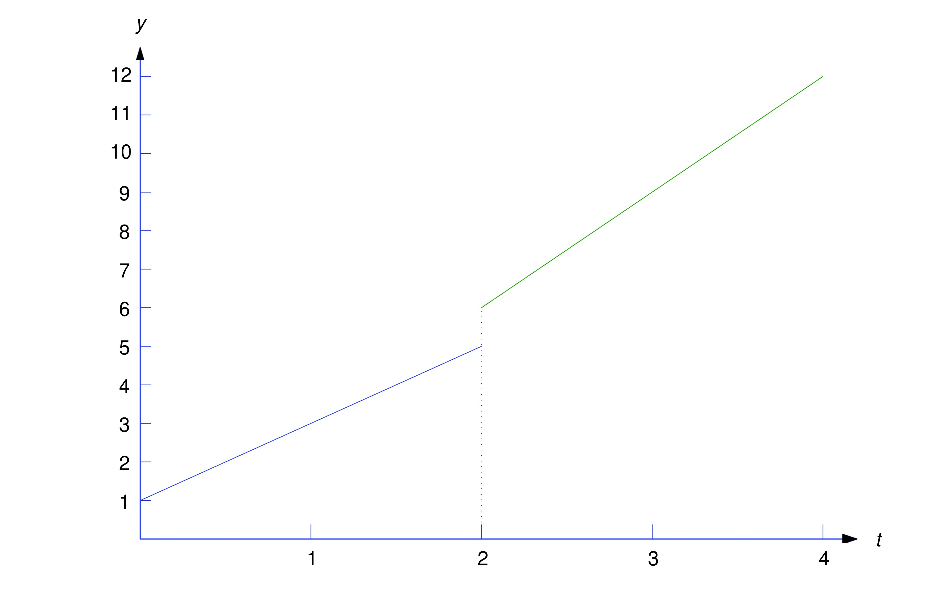
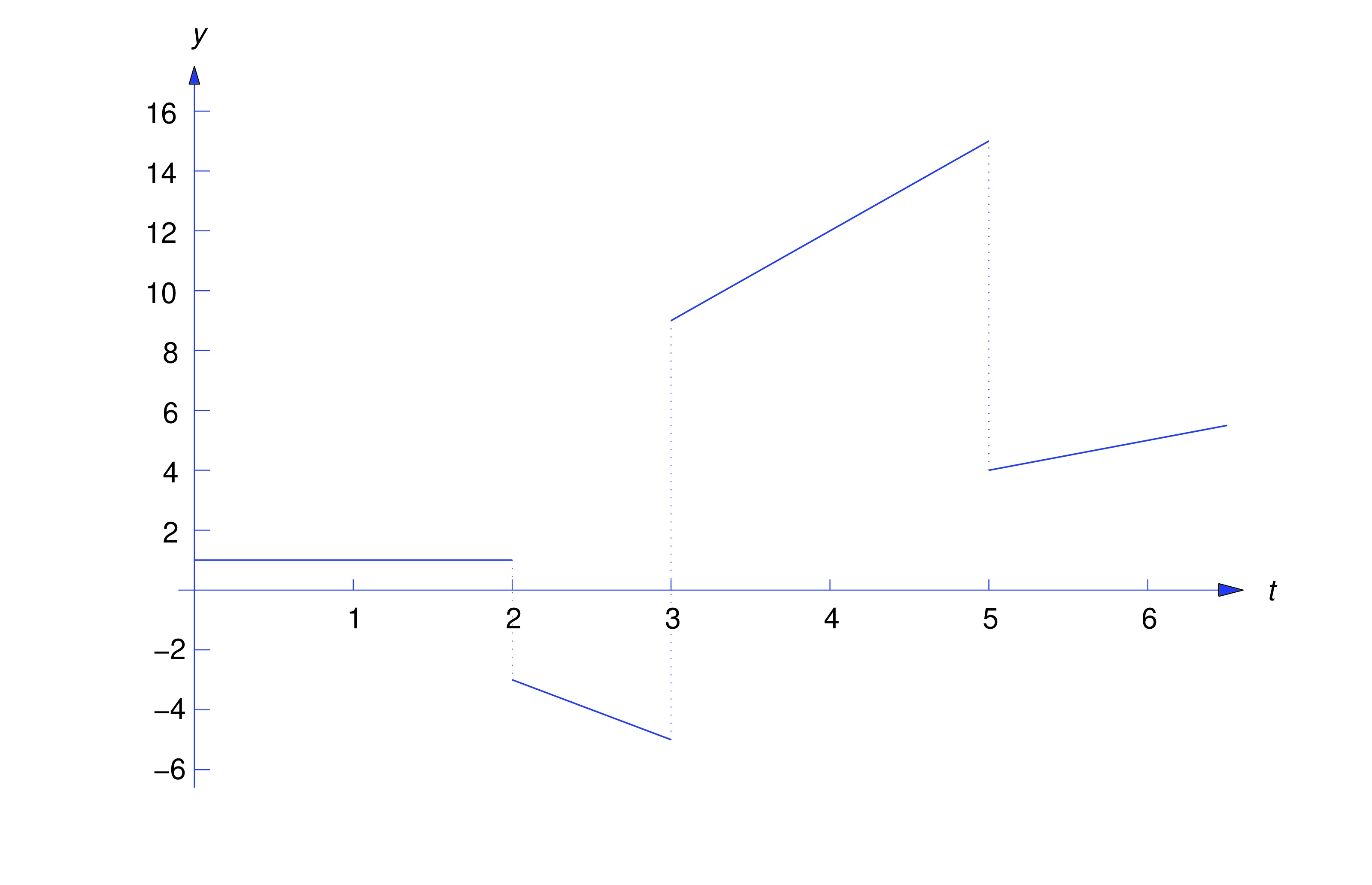
The step function enables us to represent piecewise continuous functions conveniently. For example, consider the function
where we assume that and are defined on , even though they equal only on the indicated intervals. This assumption enables us to rewrite (eq:8.4.5) as To verify this, note that if then and (eq:8.4.6) becomes If then and (eq:8.4.6) becomes
We need the next theorem to show how (eq:8.4.6) can be used to find .
Let be defined on Suppose and exists for Then exists for , and
- Proof
- By definition, From this and the definition of , The first integral on the right equals zero. Introducing the new variable of integration in the second integral yields Changing the name of the variable of integration in the last integral from to yields
Find
Here and , so Since Theorem thmtype:8.4.1 implies that
Use Theorem thmtype:8.4.1 to find the Laplace transform of the function from Example example:8.4.1.
We first write in the form (eq:8.4.6) as Therefore
which is the result obtained in Example example:8.4.1.
Formula (eq:8.4.6) can be extended to more general piecewise continuous functions. For example, we can write as if , , and are all defined on .
Find the Laplace transform of
In terms of step functions,
or Now Theorem thmtype:8.4.1 implies that
The trigonometric identities
are useful in problems that involve shifting the arguments of trigonometric functions. We'll use these identities in the next example.
Find the Laplace transform of
In terms of step functions, Now Theorem thmtype:8.4.1 implies that Since and we see from (eq:8.4.11) that
The Second Shifting Theorem
Replacing by in Theorem thmtype:8.4.1 yields the next theorem.
Second Shifting Theorem] If and exists for then exists for and or, equivalently,
Use (eq:8.4.12) to find
To apply (eq:8.4.12) we let and . Then and (eq:8.4.12) implies that
Find the inverse Laplace transform of and find distinct formulas for on appropriate intervals.
Let Then Hence, (eq:8.4.12) and the linearity of imply that
which can also be written as
Find the inverse transform of
Let and Then and Therefore (eq:8.4.12) and the linearity of imply that
Using the trigonometric identities (eq:8.4.8) and (eq:8.4.9), we can rewrite this as
Text Source
Trench, William F., "Elementary Differential Equations" (2013). Faculty Authored and Edited Books & CDs. 8. (CC-BY-NC-SA)
https://digitalcommons.trinity.edu/mono/8/
Find Particular Solution to Differential Equation With Step Function
Source: https://ximera.osu.edu/ode/main/unitStepFunction/unitStepFunction